14. Taylor Series for Approximations¶

Taylor series are commonly used in physics to approximate functions making them easier to handle specially when solving equations. In this notebook we give a visual example on how it works and the biases that it introduces.

14.1. Theoretical Formula¶

Consider a function \(f\) that is \(n\) times differentiable in a point \(a\). Then by Taylor’s theorem, for any point \(x\) in the domain of f, we have the Taylor expansion about the point \(a\) is defined as:

(14.1)¶\[\begin{equation} f(x) = f(a) + \sum_{k=1}^n \frac{f^{k}(a)}{k!}(x-a)^k + o\left((x-a)^n\right) \quad, \end{equation}\]

where \(f^{(k)}\) is the derivative of order \(k\) of \(f\). Usually, we consider \(a=0\) which gives:

(14.2)¶\[\begin{equation} f(x) = f(0) + \sum_{k=1}^n \frac{f^{k}(0)}{k!}(x)^k + o\left((x)^n\right) \quad. \end{equation}\]

For example, the exponential, \(e\) is infinitely differentiable with \(e^{(k)}=e\) and \(e^0=1\). This gives us the following Taylor expansion:

(14.3)¶\[\begin{equation} e(x) = 1 + \sum_{k=1}^\infty \frac{x^k}{k!} \quad. \end{equation}\]

14.2. Visualising Taylor Expansion Approximation and its Bias¶

Let us see visually how the Taylor expansion approximatees a given function. We start by defining our function below, for example we will consider the exponential function, \(e\) again up to order 3.

#### FOLDED CELL
%matplotlib inline
import matplotlib.pyplot as plt
from IPython.display import Markdown as md
from sympy import Symbol, series, lambdify, latex
from sympy.functions import *
from ipywidgets import interactive_output
import ipywidgets as widgets
from sympy.parsing.sympy_parser import parse_expr
import numpy as np

x = Symbol('x')

order = 3
func = exp(x)

#### FOLDED CELL
taylor_exp = series(func,x,n=order+1)
approx = lambdify(x, sum(taylor_exp.args[:-1]), "numpy")
func_np = lambdify(x, func, "numpy")
latex_func = '$'+latex(func)+'$'
latex_taylor = '\\begin{equation} '+latex(taylor_exp)+' \end{equation}'

The Taylor expansion of is :

Now let’s plot the function and its expansion while considering a point, noted \(p\), to study the biais that we introduce when we approximate the function by its expansion:

#### FOLDED CELL
text_offset = np.array([-0.15,2.])

func='exp(x)'
order = 3
x1 = 3
x_min, x_max = -4,4
func_sp = parse_expr(func)
taylor_exp = series(func_sp,x,n=order+1)
approx = lambdify(x, sum(taylor_exp.args[:-1]), "numpy")
func_np = lambdify(x, func_sp, "numpy")
n_points = 1000
x_array = np.linspace(x_min,x_max,n_points)
approx_array = np.array([approx(z) for z in x_array])
func_array = np.array([func_np(z) for z in x_array])
func_x1 = func_np(x1)
approx_x1 = approx(x1)
plt.figure(42,figsize=(10,10))
plt.plot(x_array,approx_array,color='blue',label='Taylor Expansion')
plt.plot(x_array,func_array,color='green',label=func)
plt.plot(0,approx(0),color='black',marker='o')
plt.annotate(r'(0,0)',[0,approx(0)],xytext=text_offset)
plt.plot([x1,x1]
         ,[-np.max(np.abs([np.min(func_array),np.max(func_array)])),min(approx_x1, func_x1)]
         ,'--',color='black',marker='x')
plt.plot([x1,x1],[approx_x1, func_x1],'r--',marker='x')
plt.annotate(r'$p_{approx}$',[x1,approx(x1)],xytext=[x1,approx(x1)]-text_offset)
plt.annotate(r'$p$',[x1,func_np(x1)],xytext=[x1,func_np(x1)]-text_offset)
plt.xlim([x_min,x_max])
plt.ylim(-np.max(np.abs([np.min(func_array),np.max(func_array)]))
         ,np.max(np.abs([np.min(func_array),np.max(func_array)])))
plt.legend()
plt.show()
print('Approximation  order : {}'.format(order))
print('Approximation  bias  : {}'.format(func_x1-approx_x1))

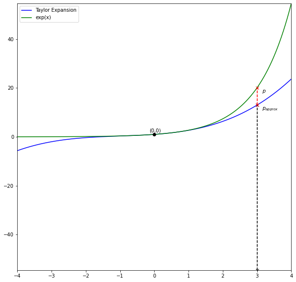
Approximation  order : 3
Approximation  bias  : 7.085536923187668

Notice that the further \(p\) gets away from the point of the expansion (in that case \(0\)), the higher the approximation bias gets. Samely, the lower the order of approximation is, the higher the approximation bias gets.

Shear Book

14. Taylor Series for Approximations¶

14.1. Theoretical Formula¶

14.2. Visualising Taylor Expansion Approximation and its Bias¶