6.2. Contributors to the PSF
6.2.1. Optic level
Mirrors
Aberrations
There are imperfections in the curvature of mirrors producing different types of aberrations. These introduce optical path differences for the incoming light rays producing features in the PSF.
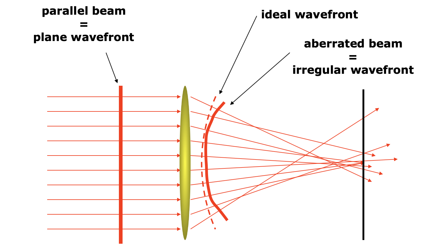
Fig. 6.1 Illustration of the optical path differences in a lens. Note that current telescopes are build with mirrors but the illustration shows a lens. Credit: Austin Roorda.
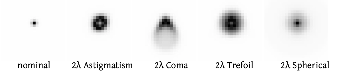
Fig. 6.2 Typical aberrations with simulated in-focus stars with typical seeing. Credit: Aaron Roodman.
Mirrors
Size
The size of the main mirror has a direct implicance to the size of the PSF. Following the diffraction theory, the larger the mirror for the lens, the smaller size the PSF should have. There are practical limitations on the maximal sizes of mirrors that are due to the manufacturing process.
Polishing effects
The polishing of the mirrors aims to have a perfectly smooth surface. However, the manufacturing process is not perfect and small errors remain in the surface of the mirrors. They are sometimes referred to as surface errors.
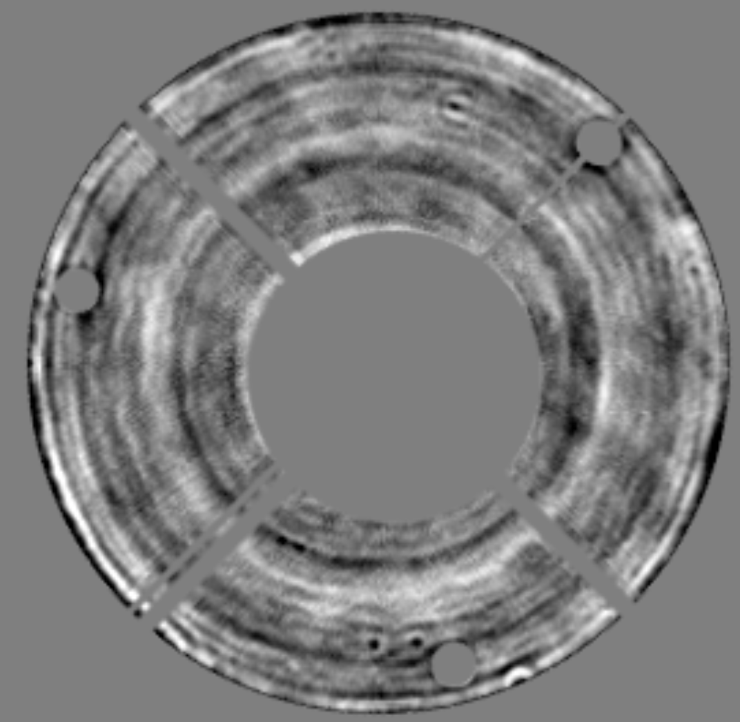
Fig. 6.3 Surface errors estimated for the Hubble Space Telescope. They are in the range of +/- 30nm. Credit: [KHS11].
Optical system
Misalignment
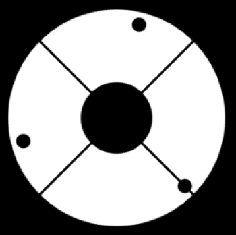
Misalignement of optical elements can cause a defocus of the system. For example, in Figure 7 and 8 from [JT11] one can see the effects of Charge-Coupled Devices (CCD) misalignements on the focal plane on a simulation of the LSST mission [LSSTSCollaborationAbellAllison+09].
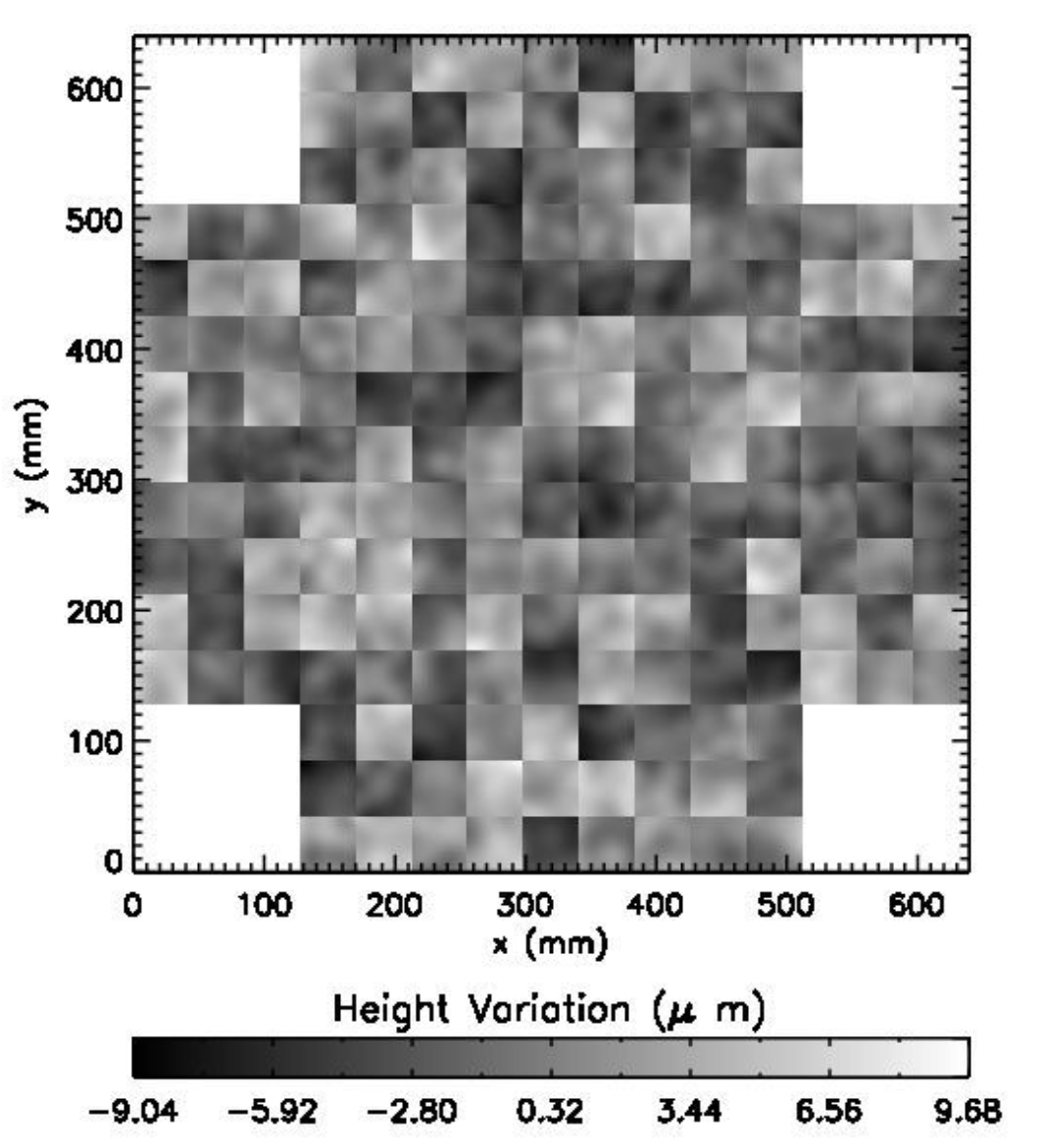
Fig. 6.4 Simulated focal plane of LSST. We used the CCD assembly/fabrication specification in Table 1 to generate the LSST focal plane tiled by 189 CCDs. Credit: [JT11].
Optical system
Scattered light
It consist of spuriours reflections within the optical system and the detector. An example for the HST mission can be found in Fig 3 in [Kri95].
Optical system
Wavelength dependency
The optical system is composed by several elements where some of them can be non-ideal refractive elements. This means that they introdcuce a wavelength dependance variation.
Obscurations
Depending on the optical system design it might require arms to sustain the camera or even superposing mirrors that block each other. These obscurations modify the shape of the PSF and vary depending on the source’s angle of incidence. They are 3D structures that are projected on the 2D pupil plane.
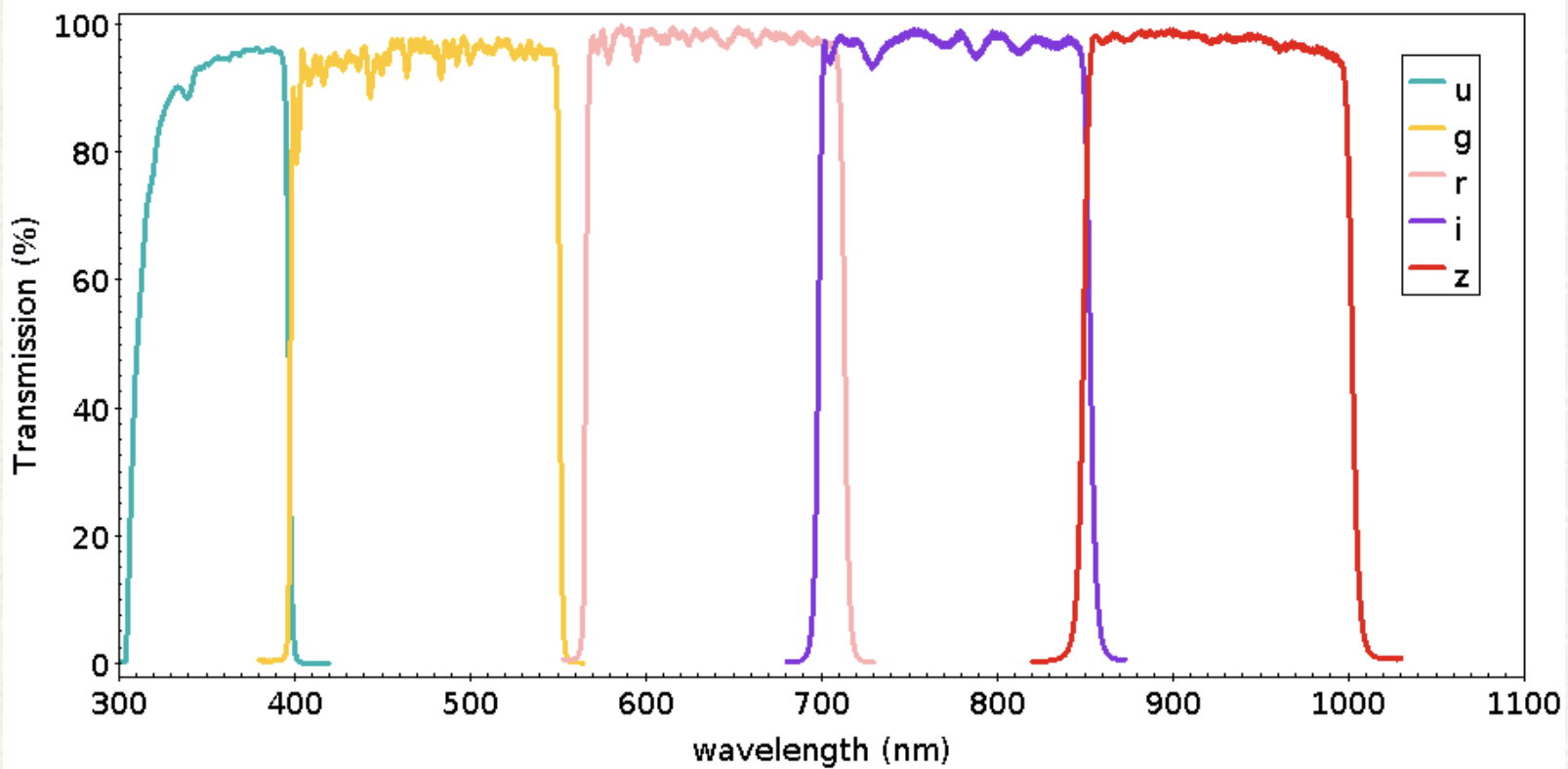
Filters
Passband
The filters serve to select the wavelengths incoming to the detector. Ideally they would be a perfect band-pass filter, begin one at the desired wavelength range and zero on the other wavelengths. However, it is not possible to manufacture an ideal filter. A real one does not have an abrupt transition, meaning that there are out-of-band contributions. It is also non-flat, meanining that the passband is near the unity but it changes with the wavelength. See this page to visualise some examples of filters.
6.2.2. Ground-based
Atmosphere
The atmosphere plays a central role in ground-based observations. The refractive index of the atmosphere varies rapidly with the position generating different optical paths for the incoming light. As a consequence, the way it affects the PSF changes if we consider short-term exposures or long-term exposures. It also depends of the incoming wavelength. See [JT11] for a first study on the Legacy Survey of Space and Time (LSST) from the Vera C. Rubin Observatory.
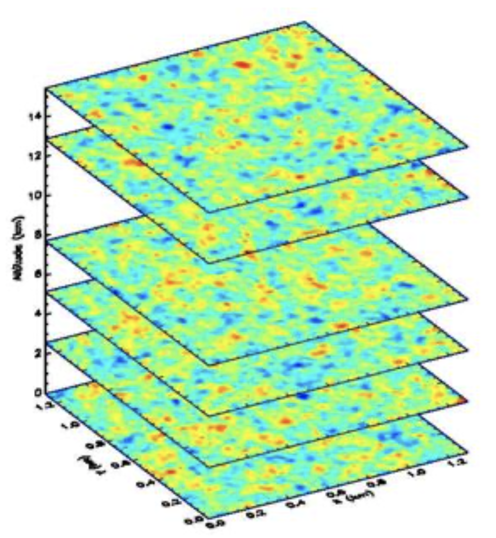
Fig. 6.7 Six layers of Kolmogorov/von Karman phase screens used for the atmospheric turbulence model. These phase screens represent the variations of the refractive index for different heights in the atmosphere. Credit: [JT11].
Observing environment
The temperature differences in the telescope environment as well as the wind speed and direction on the surroundings of the telescope can affect its image quality. See [SCB+09] for a study on the Canada-France-Hawaii Telescope (CFHT).
6.2.3. Space-based
Guiding errors
The satellite should remain perfectly still during an exposure. This is not the case and there exist a pointing error making the exposure the integration of the varyign satellite pointing. It sometimes referred as Jitter or Attitude and Orbit Control System.
Thermal variations
The satellite experiences time where the sun is closer or were it is eclipsed by other object. This can occasionate high temperature changes in the space telescope. These temperature variations dilate and contract the optical system making it change of state as a function of temperature. It is sometimes to as telescope’s breathing for its repetitive pattern due to the orbits. See [NML+07] for an HST study of temperature variations.
Polarisation
Starlight can be naturally polarised by galactic foreground dust. The different polarisations that the incoming light has can interact differently with refractive elements of the optical system. This occasionates variations that are polarisation dependent. This source is currently being studied.
6.2.4. Detector level
Undersampling and pixelation
Many detectors, specially space-based ones, are undersampled or not Nyquist sampled. Generally, several exposures of the same object with small shifts are taken in order to super-resolve the object. The pixelation effect, the fact of using a limited number of pixels also affects the PSF and will impact the shear measurements. See [HRME07] for a study of pixelation effects in weak lensing. See Section 3.5 and Figure 4 from [KHS11] for an analysis of these effects on the HST telescope.
Fig. 6.10 On top, the computed 336 nm HST PSF prior to pixellation. Below it is the PSF centered at the middle of a pixel and in the corner, integrated over the WFPC2 WF pixel area, shown at the same spatial scale. Credit: [KHS11].
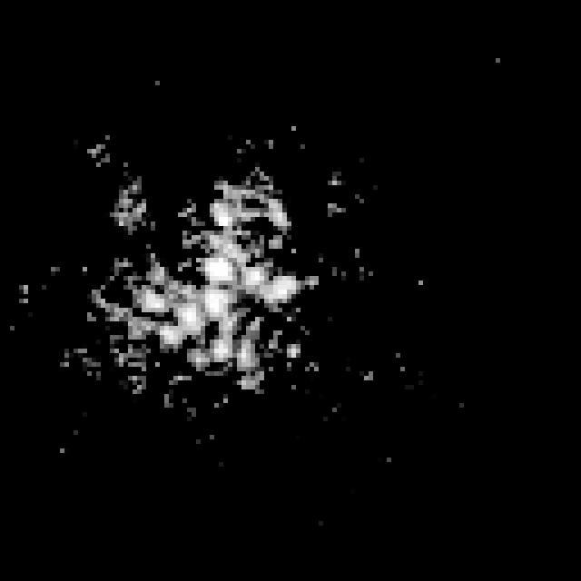
Charge Diffusion Effect
There is a charge diffusion of the electrons between the pixels. It depends on the depth of the substrate and on the wavelength. It varies in the field of view as seen in [Kri03] on a study for the HST mission. It can be modelled as a varying convolutional kernel.
Fig. 6.11 Surface fits to the measured WFC charge diffusion blur kernel widths shown over the entire field of view (WFC1 & WFC2 butted together). The images are scaled to the same linear range. Credit [Kri03].
Charge Transfer Inefficiency
Brighter Fatter Effect
Each pixel in an camera is not independent of each other. One charge starts accumulating it modifies boundary pixel’s electric fields. This occasionates a variation of the PSF size as a function of the flux and the wavelength. See [GAA+15] for a study and a model of the effect.
Quantum efficiency
This effect describes the ratio of created electrons from the number of incoming photons. It depends on the wavelength and on the detector’s technology.
Other effects
Analog-to-Digital Unit non-linearity
Thermal noise
Background estimation and subtraction