10.1. KSB¶

In this section, we introduce the Kaiser-Squire-Broadhurst method (KSB) to measure galaxies shape using the image of the galaxy surface brightness.

KSB estimates the reduced shear \(g\) using the polarisation \(\chi\). The exact relation between these quantities is :

(10.1)¶\[ \chi^s = \frac{\chi - 2 g +g^2 \chi^\ast}{1 + | g |^2 - \Re \left( g \chi^\ast \right) } \quad, \]

where \(\chi^s\) is the intrinsic (unlensed) polarisation.

Assuming that the average of \(\chi^s\) vanishe, i.e. \(\left< \chi^s \right>=0\), and in a certain region \(g\) is constant, \(g\) is approximated by rotating the coordinate frame such that only one of its component does not vanish:

\[ g \approx \frac{ \left< \chi \right> }{ 2 \left(1 - \sigma^2_\chi\right) } + \frac{\left< \chi \right>^3}{8} \frac{1 - 5\sigma^2_\chi}{ \left(1 - \sigma^2_\chi\right)^4} + \mathcal{O} \left( \left< \chi \right>^5 \right) \quad, \]

with \(\sigma^2_\chi\) being the standard deviation of \(\chi^s\) distribution.

Note

The polarisation \(\chi\) is used for shear measurement instead of the ellipticity \(\epsilon\) in Weak Lensing because in practice its estimator is less noisy.

Warning

The approximation of \(g\) is done by applying a Taylor Expansion of \(\chi\) around 0, i.e. for small value of \(\chi\), on the average of (10.1).

10.1.1. Standard KSB¶

The core idea of KSB is to deduce the reduced shear by estimating the polarisation on raw data, i.e. images blurred by a known PSF and contaminated with additive Gaussian noise, and using a weighting window on each image then apply corrections directly in the polarisation space.

In the following, the PSF effect and the weighting window effect are handled separately.

10.1.1.1. Handling the Weighting Window¶

Here the polarisation \(\chi\) is estimated using the weighted moments \(Q_w\) and \(\chi^s\) is the unaccessible polarisation of the source observed by a perfect telescope (no PSF effect) and without any noise.

By introducing the shear polarisability matrix, \(P^{sh}\), a first order approximation in terms of \(g\) gives :

(10.2)¶\[ \chi - \chi^s = P^{sh} g \]

with

\[ P^{sh}_{\alpha \beta} = - 2 \frac{\chi_{\alpha}L_{\beta}}{Q_{w,xx}+Q_{w,yy}} - 2 \chi_{\alpha}\chi_{\beta} + 2 \frac{B_{\alpha \beta}}{Q_{w,xx}+Q_{w,yy}} + 2 \delta_{\alpha \beta} \]

such that \(\alpha, \beta \in \{1,2\}\) the indices of the components and \(\delta_{\alpha \beta}\) is the Kronecker delta and

\[ L_\beta = \frac{1}{\sigma^2} \sum_{x,y} I(x,y) W'\left(\frac{(x,y)}{\sigma}\right) \eta_\beta \]

\[ B_{\alpha \beta} = \frac{1}{\sigma^2} \sum_{x,y} I(x,y) W'\left(\frac{(x,y)}{\sigma}\right) \eta_\beta \eta_\beta \]

where \(W\) is the weighting window function and \(\sigma\) its scaling factor along with

\[ \eta_1 = x^2 - y^2 \]

and

\[ \eta_2 = 2xy. \]

By averaing equation (10.2), \(\left<\chi^s\right> = 0\) (no intrinsic alignment assumption), \(\left<g\right> = g\) (weak lensing assumption) and by multplying both sides by \(\left<P^{sh}\right>^{-1}\), we obtain:

(10.3)¶\[ g = \left<P^{sh}\right>^{-1}\left< \chi \right> \]

Equation (10.3) applies when the all the sources have locally constant morphology and size. In practice, this does not hold because the sources are affected by the PSF which adds instability to the morphology and size. Commonly in cosmic-shear, the averages are interchanged:

(10.4)¶\[ \left< \tilde{g} \right> = \left< \left(P^{sh}\right)^{-1} \chi \right> \]

with the assumption that \(\left< \left( P^{sh}\right)^{-1} \chi^s \right> = 0\) which does not hold in reality because \(P^{sh}\) depends on \(\chi\).

Nevertheless, \(\tilde{g}\) is the solution to (10.2) with \(\chi^s=0\). This corresponds to the shear of a circular source. The tru value of \(g\) is obtained by averaging \(\tilde{g}\).

10.1.1.2. Handling the PSF Effect¶

In KSB the PSF is supposed to be almost istropic and its effects on the source polarisation are linearly modelled by:

\[ \chi = \chi^{obs} + \chi^{g} \]

where \(\chi\) is the polarisation that would have been observed without the PSF effect (it is the same \(\chi\) from the section above), \(\chi^{obs}\) is the polarisation observed by the telescope and \(\chi^g\) contains the effects of the PSF which expression is:

\[ \chi^g = P^{sm} \left( P^{sm,*}\right)^{-1} \chi^{sh,*} \]

\(P^{sm}\) is the smear polarizability matrix and it accounts for the effects of the isotrpic part of the PSF, \(P^{sm,*}\) and \(\chi^{sh,*}\) are respectively the smear polarizability and the polarization of a star and are used to account for the anisotropies of the PSF that are supposed to be small. The star is supposed to give an empirical estimation of the PSF near the source. The expression of the smear polarizabilty is:

\[ P^{sm}_{\alpha \beta}=\frac{1}{Q_{xx}+Q_{yy}}\left[ \left( M + 2\frac{Q'_{xx}+Q'_{yy}}{\sigma^2} \right) \delta_{\alpha \beta} + G_{\alpha \beta} -\chi_\alpha \left( 2 F_\beta + L'_\beta \right) \right] \]

where \(L'_\alpha\) is equivalent to \(L_\alpha\) calculated with the second order derivative of the weighting window function, \(Q'_{k,k}\) (with \(k \in {x,y}\)) is equivalent to the moments weighted by the first order derivative of the weighting window function and

\[ M = \sum_{x,y} I(x,y) W \left( \frac{\left(x,y\right)}{\sigma} \right) \quad, \]

\[ F_\alpha = \frac{1}{\sigma^2}\sum_{x,y} I(x,y) W' \left( \frac{\left(x,y\right)}{\sigma} \right) \eta_\alpha \quad, \]

\[ G_{\alpha \beta} = \frac{1}{\sigma^4} \sum_{x,y} I(x,y) W'' \left( \frac{\left(x,y\right)}{\sigma} \right) \eta_\alpha \eta_\beta \quad. \]

10.1.1.3. KSB in practice¶

The reduced shear is estimated by removing the PSF effect then solving equation (10.4).

The original KSB [KaiserSquiresBroadhurst95] had an incorrect approximation of \(g\). Many ameliorations were suggested, namely from [ViolaMelchiorBartelmann11] which pushed the approximations up to the third order. Alternative methods to KSB exist, for example there is the re-Gaussianization approach which is used in HSC [HirataSeljak03].

First order approximation and limited Taylor expansion induce a large bias for the points that are distant from the expansion point, for more details see the appendix on Taylor series. This means that for high values of \(g\) the error is more important than for smaller values, as seen in the figure below.

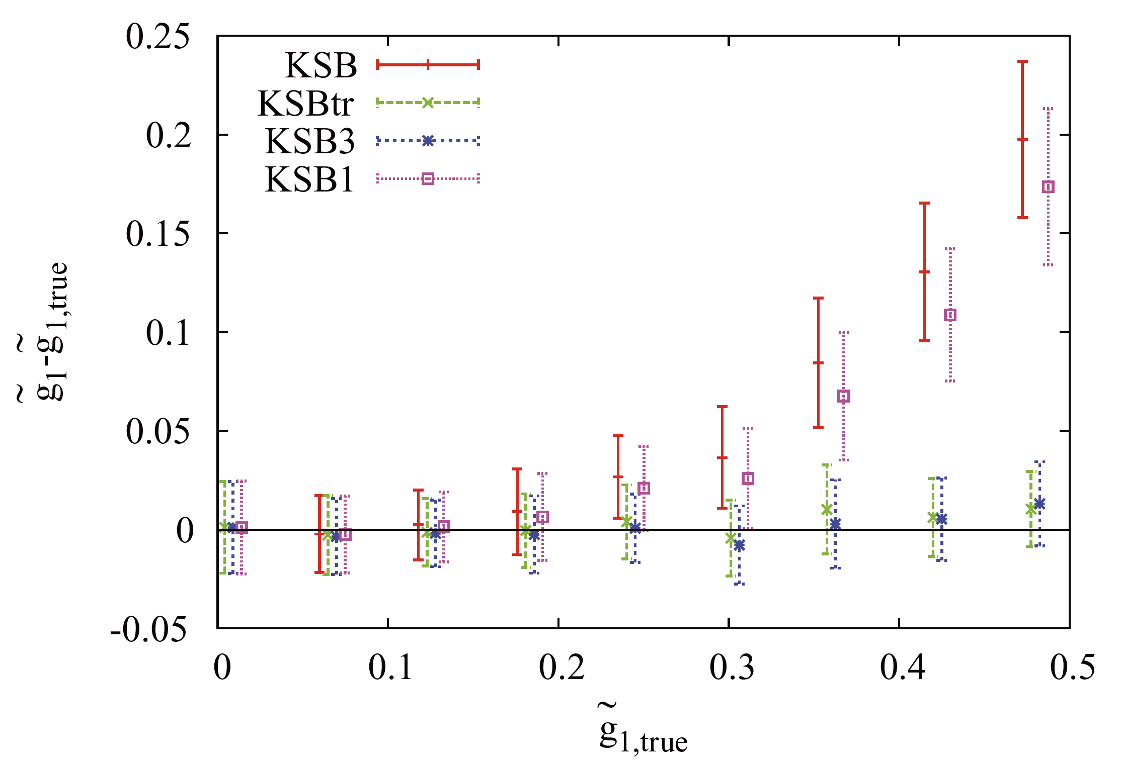
Fig. 10.1 Shear estimation for unconvolved and almost noiseless galaxies with Sersic profile. KSB (red solidline) goes to third order approximations which are incorrect, KSB1 (violet dotted) is a first order approximation, KSBtr (green long-dashed line) is a third order approximation that is not mathematically justified and KSB3 (blue short-dashed line) is the correct third order approximation. Source [ViolaMelchiorBartelmann11].¶

Also KSB works under the hypothesis that the PSF has small anisotropies which is not always the case, specially in Radio Interferometry for example.

Furthermore, the correction of the weighting window effect is approximative which adds another bias to the estimation of \(g\) that depends on the choice of the window parameters (e.g. \(\sigma\)).

Finally, a C++ implementation of KSB by Peter Melchior can be found on this GitHub repository. And in the following code snippet, an example of how to use the GalSim KSB implementation to estimate the shear of a galaxy contained in image which was convolved by psf (assuming that both image and psf are numpy arrays):

import galsim
from galsim import Image
import galsim.hsm

#set pixel scale
scale = 0.1
#create a galsim version of the data
image_galsim = Image(image,scale=scale)
psf_galsim = Image(psf,scale=scale)
#estimate the moments of the observation image
ell=galsim.hsm.EstimateShear(image_galsim
                             ,psf_galsim,shear_est='KSB')

Shear Book