ShapePipe Tutorial
Contents
ShapePipe Tutorial
Quick start
Run the entire pipeline on a single example CFIS image with tile ID 246.290:
Install
ShapePipeand activate theshapepipeconda environment.Run the job script
job_sp 246.290 -j 127
Introduction
The ShapePipe pipeline processes single-exposure images and stacked images. Input images have to be calibrated beforehand for astrometry and photometry. This tutorial of an entire ShapePipe run covers specifically images from CFIS, the Canada-France Imaging Survey. CFIS stacks are so-called tiles, which are the co-adds of on average three exposures in the r-band.
File types and names
The ShapePipe pipeline handles different image and file types, some of which
are created by the pipeline during the analysis. These file types are listed below.
All files follow a (configurable) naming and numbering convention, to facilitate bookkeeping for
tracking relevant image information. In general, the convention is <image_type>_ID can be a combination of numbers and special characters such as -.
Naming and numbering of the input files can closely follow the original image names and (ID) numbers provided by the telescope and pre-processing software, with some required modifications as described below.
Single-exposure mosaic image.
Multi-HDU FITS file containing a mosaic from multiple CCDs of a single exposure (an exposure is also called epoch). Each CCD is stored in a different HDU. These files are used on input byShapePipe. The pixel data can contain the observed image, a weight map, or a flag map. These images are typically created by a telescope analysis software (e.g.~pitcairn). Examples from CFIS are2228303p.fits.fz,2214439p.flag.fits.fz. These names need to be modified to be correctly identified byShapePipe: Thepneeds to be removed, the image type needs to precede the ID, and the file name can only contain a single dot (.) delimiting the file extension. We create the extensionfitsfzfor compressed FITS file.
Default convention: <image_type>-<exposure_number>.fitsfz.
Examples:image-2228303.fitsfz,flag-2214439.fitsfzSingle-exposure single-CCD image.
FITS file containing a single CCD from an individual exposure. The pixel data can contain the observed image, a weight map, or a flag map.
Default convention: <image_type>-<exposure_number>-<CCD_number>.fits
Examples:image-2079614-9.fits,weight-2079614-3.fitsStacked images
FITS file containing a stack by co-adding different single exposures, created by software such asswarp. A stacked image is also called tile. These files are used on input byShapePipe. The pixel data can contain the observed image, a weight map, or a flag map. Tile images and weights are created in the case of CFIS by Stephen Gwyn using a combination ofswarpand his own software. Examples of file names areCFIS.316.246.r.fits,CFIS.205.267.r.weight.fits.fz, the latter is a compressed FITS file, see below. Tile flag files are created the mask module ofShapePipe(see Mask images). The tile ID needs to be modified such that the.between the two tile numbers (RA and DEC indicator) is not mistaken for a file extension delimiter. For the same reason, the extension.fits.fzis changed to.fitzfz. In addition, for clarity, we include the stringimagefor a tile image type.
Default convention: <image_type>-<tile_number>.fits
Examples:CFIS_image-277-282.fits,CFIS_weight-274-282.fitsfz,pipeline_flag-239-293.fitsDatabase catalogue files
For very large files that combine information from multiple tiles or single exposures,ShapePipecreatessqlitedata base catalogues.
Examples:log_exp_headers.sqlite, exposure header informationNumpy array binary files
Some large files are stored as numpy arrays. These contain FITS header information. Example:headers-2366993.npyPSF files
PSFExandSExtractorproduce FITS files with file exentions other than.fits:.psffor files containing PSF model information for a single CCD, and.catfor a PSF catalogue.final shape catalogue The end product of
ShapePipeis a final catalogue containing a large number of information for each galaxy, including its shape parameters, the ellipticity components :math:e_1and :math:e_2. This catalogue also contains shapes of artificially sheared images. This information is used in post-processing to compute calibrated shear estimates via metacalibration.Summary statistic files
TheSEToolsmodule that creates samples of objects according to some user-defined selection criteria (see Select stars) also outputs ASCII
files with user-defined summary statistics for each CCD, for example the number of selected stars, or mean and standard deviation of their FWHM.
Example:star_stat-2366993-18.txtTile ID list
ASCII file with a tile number on each line. Used for theget_image_runnermodule to download CFIS images (see Download tiles).Single-exposure name list
ASCII file with a single-exposure name on each line. Produced by thefind_exposure_runnermodule to identify single exposures that were used to create a given tile. See Find exposures).Plots
TheSEToolsmodule can also produce plots of the objects properties that were selected for a given CCD. The type of plot (histogram, scatter plot, …) and quantities to plot as well as plot decorations can be specified in the selection criteria config file (see Select stars). Example:hist_mag_stars-2104133-5.pngLog files
The pipeline core and all called modules write ASCII log files to disk.
Examples:process-2366993-6.log,log_sp_exp.log.
CFIS processing
ShapePipe splits the processing of CFIS images into several parts:
These are the retrieval and preparation of input images, processing of single exposures,
processing of tile images, creation and upload (optional) of final shape catalogues.
The following flowchart visualised the processing parts and steps.
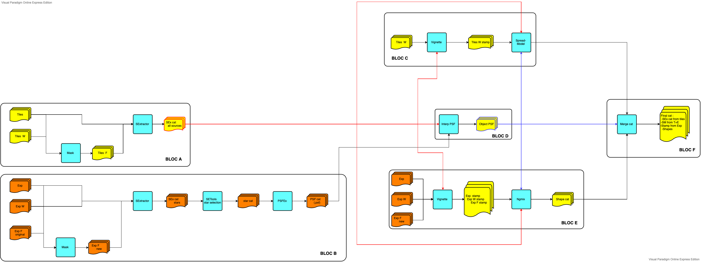
Below, the individual processing steps are described in detail.
Input and output paths
All required paths are automatically set in the job script job_sp.
If an example config file is run outside this script, the following path variables might need to be defined.
$SP_RUN: Run directory ofShapePipe. In general this is justpwd, and can be set viaexport SP_RUN=`pwd`
but on a cluster this directory might be different.
$SP_CONFIG: Path to configuration files. In our example this is$SP_BASE/example/cfis.
In addition, the output path $SP_RUN/output needs to be created by the user before running ShapePipe.
Job and pipeline scripts
The job script to run the pipeline in its entity or in parts is job_sp[.bash]. Type
job_sp -h
for all options.
This script creates the subdirectory $SP_RUN/output to store all pipeline outputs
(log files, diagnostics, statistics, output images, catalogues, single-exposure headers with WCS information).
Optionally, the subdir output_star_cat is created by the used to store the external star catalogues for masking. This is only necessary if the pipeline is run on a cluster without internet connection to access star catalogues. In that case, the star catalogues need to be retrieved outside the pipeline, for example on a login node, and copied to output_star_cat.
The job script automaticall performs a number of subsequent calls to the ShapePipe executable shapepipe_run, as
shapepipe_run -c $SP_CONFIG/<config>.ini
The config file <config>.ini contains the configuration for one or more modules.
See the main ShapePipe readme for more details.
The user specifies which steps are run with the command line option -j JOB. The integer value JOB
is bit-coded such that arbitrary combinations of steps can be run with a single call to job_sp. For
example, to run steps #1 and #2, type job_sp -j 3.
Select tiles
To run the job script, one or more CFIS tiles need to be chosen. If the tile IDs are known, they are provided to job_sp on the command line.
If the tile IDs are not known a priori, they can be selected via sky coordinates, with the script cfis_field_select.
For example, to find the tile number for a Planck cluster at R.A.=213.68 deg, dec=57.79 deg, run:
cfis_field_select -i /path/to/shapepipe/auxdir/CFIS/tiles_202007/tiles_all_order.txt --coord 213.68deg_54.79deg -t tile --input_format ID_only --out_name_only --out_ID_only -s
The input text file (provide via the flag -i) contains a list of CFIS tiles, this can also be directory containing the tile FITS files.
The following sections describe the different steps that are performed with job_sp.
Run the pipeline
Retrieve input images
The command
job_sp TILE_ID -j 1
retrieves the image and weight corresponding to TILE_ID using the module get_images.
It then identifies the exposures that were used to create the tile image via the find_exposures runner.
Finally, another call to get_images retrieves the exposure images, weights, and flag files.
For the retrieval method the user can choose betwen
download from VOspace (
-r vos);create symbolic link to existing file on disk (
-r symlink).
Note that internet access is required for this step if the download method is vos.
An output directory run_sp_GitFeGie (in output) is created containing the results of get_images for tiles (Git),
find_exposures (Fe), and get_images for exposures (Gie).
Prepare input images
With
job_sp TILE_ID -j 2
the compressed tile weight image is uncompressed via the uncompress_fits module. Then, the single-exposure images, weight, and flags are split into single-exposure single-CCD file
(one FITS file per CCD) with split_exp.
Finally, the headers of all single-exposure single-CCD files are merged into a single sqlite file, to store the WCS information of the input exposures.
Two output directories are created, run_sp_Uz for uncompress_fits, and run_sp_exp_SpMh for the output of the modules
split_exp (Sp) and merge_headers (Mh).
Mask images
Run
job_sp TILE_ID -j 4
to mask tile and single-exposure single-CCD images. Both tasks are performed by two calls to the mask runner.
Note that internet access is required for this step, since a reference star catalogue is downloaded.
The output of both masking runs are stored in the output directory run_sp_MaMa, with run 1 (2) of
mask corresponding to tiles (exposures).
Diagnostics: Open a single-exposure single-CCD image and the corresponding pipeline flag
in ds9, and display both frames next to each other. Example
ds9 image-2113737-10.fits pipeline_flag-2113737-10.fits
Choose zoom fit for both frames, click scale zscale for the image, and color aips0 for the flag, to display something like this:
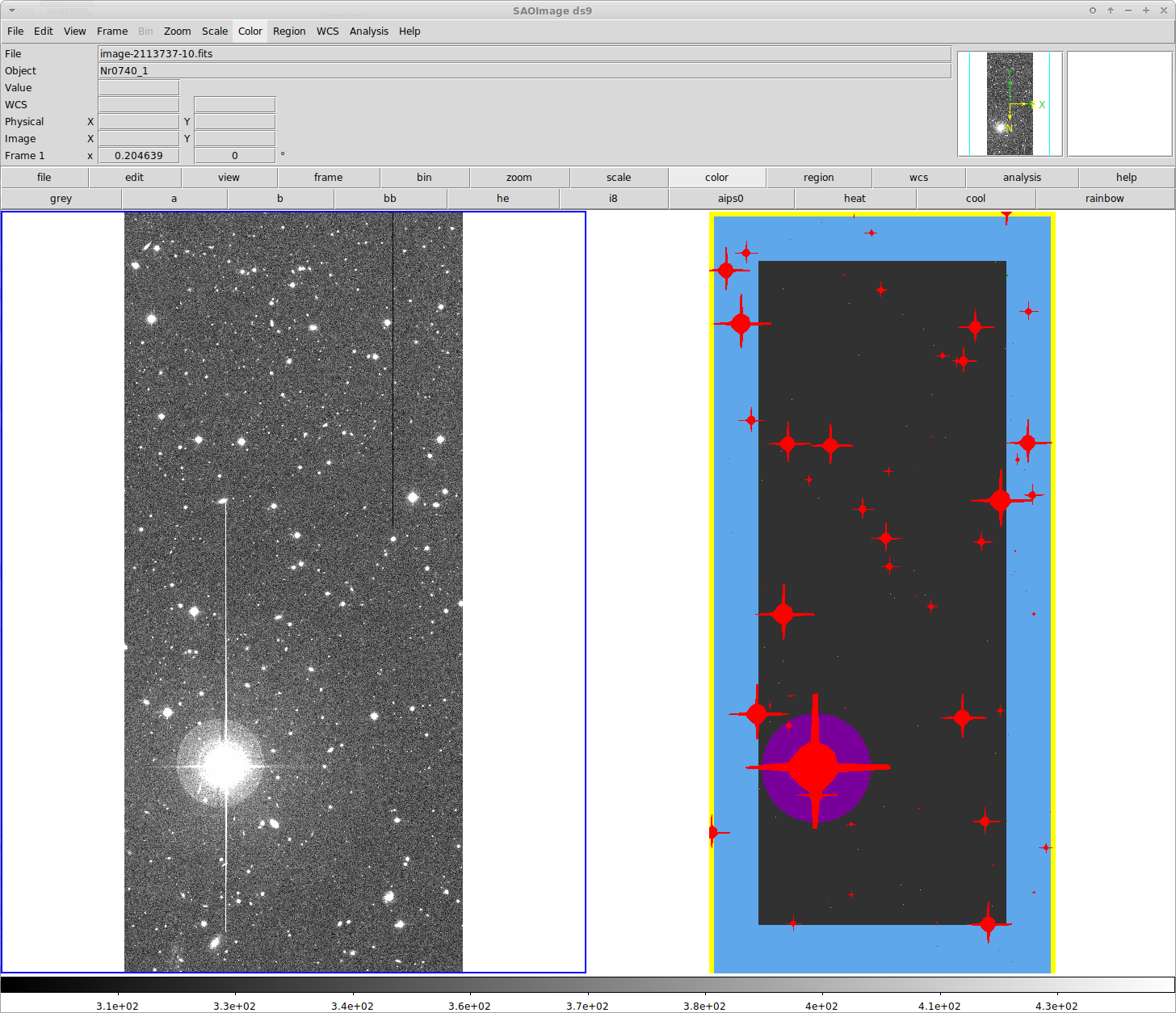
By eye the correspondence between the different flag types and the image can be
seen. Note that the two frames might not match perfectly, since (a) WCS
information is not available in the flag file FITS headers; (b) the image can
have a zero-padded pixel border, which is not accounted for by ds9.
Detect objects on tiles and process stars on single exposures
The call
job_sp TILE_ID -j 8
performs a number of steps. First, objects on the tiles are deteced with the sextractor runner.
Next, the following tasks are run on the single-exposure single-CCD images:
Objects are deteced with
sextractor.Star candidates are selected via
setools.The PSF model is created, either with
psfexfor PSFex, or withmccd_preprocessingandmccd_fit_valfor MCCD.The PSF model is interpolated to star positions for validation. For the PSFEx model, this is done via a call to
psfex_interp. For MCCD, the modulesmerge_starcat,mccd_plots, andmccd_interpare called.
The output directory for both the mccd and psfex options is run_sp_tile_Sx_exp_SxSePsf.
This stores the output of SExtractor on the tiles (tile_Sx), on the exposures (exp_Sx),
setools (Se), and the Psf model (Psf).
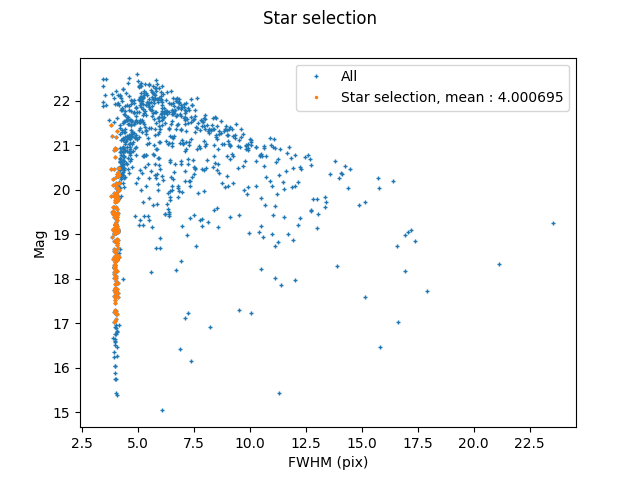
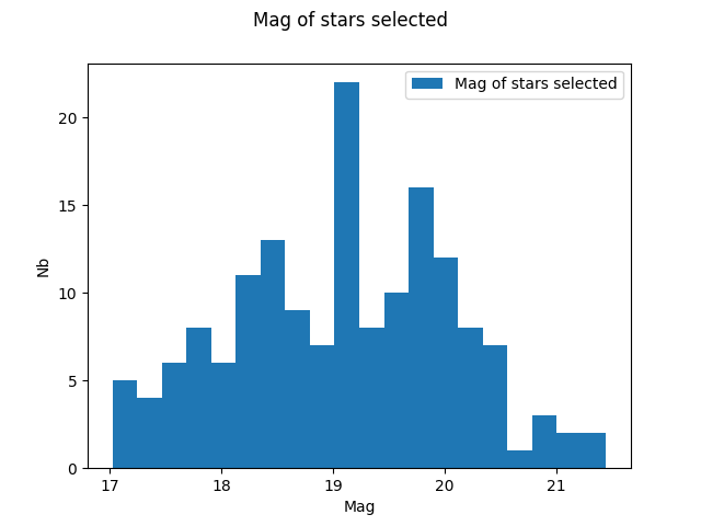
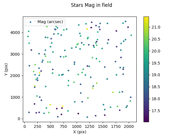
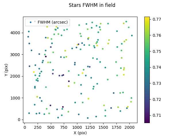
The following plots show an example of a single CCD, in the center of the focal plane.
Size-magnitude plot |
Star magnitude histogram |
Stars in CCD (mag) |
Stars in CCD (size) |
|---|---|---|---|
|
|
|
|
The stellar locus is well-defined |
Magnitude distribution looks reasonable |
Stars are relatively homogeneously distributed over the CCD |
The uniform and small seeing of CFHT is evident |
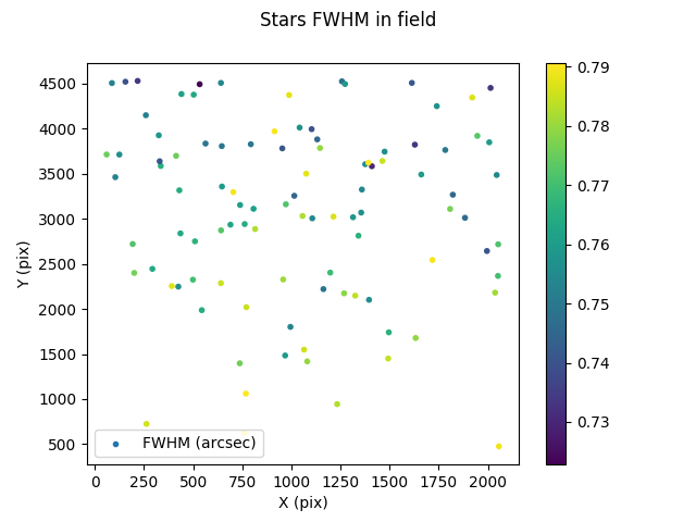
To contrast the last plot, here is the case of the CCD in the lower right corner, which shows a known (but yet unexplained) lack of stars in the lower parts:
The statistics output file for the center CCD #10:
cat star_stat-2113737-10.txt
# Statistics
Nb objects full cat = 1267
Nb stars = 160
stars/deg^2 = 6345.70450519073
Mean star fwhm selected (arcsec) = 0.7441293125152588
Standard deviation fwhm star selected (arcsec) = 0.014217643037438393
Mode fwhm used (arcsec) = 0.7345179691314697
Min fwhm cut (arcesec) = 0.7159179691314698
Max fwhm cut (arcsec) = 0.7531179691314697
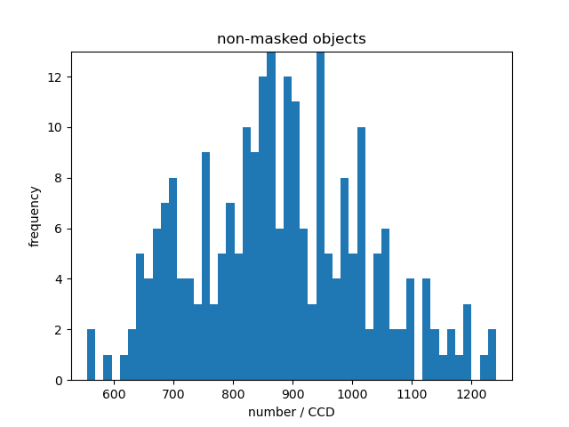
Global star sample statistics
The statistics on stars from all CCD can be combined to create histograms, with the non-pipeline script stats_global.py.
Run
stats_global -o stats -v -c $SP_CONFIG/config_stats.ini
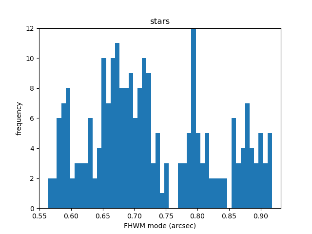
to create histograms (as .txt tables and .png plots) in the directory stats. Here are some example plots :
Non-masked objects per CCD |
Stars per CCD |
FWHM mode |
|---|---|---|
|
|
|
No CCD with a very large masked area |
No CCD with insufficient stars |
Rather broad seeing distribution |

Note that stats_global read all SETool output stats files found in a given input directory tree. It can thus produce histogram combining
several runs.
Galaxy selection
The focus of the next step,
job_sp TILE_ID -j 16
is the selection of galaxies as extended objects compared to the PSF.
First, the PSF model is interpolated to galaxy positions, according to the PSF model
with psfex_interp or mccd_interp. Next, postage stamps around galaxies
of the weights maps are created via vignetmaker. Then, the spread model
is computed by the spread_model module. Finally, postage stamps
around galaxies of single-exposure data is extracted with another call
to vignetmaker.
The output directory is
run_sp_MiViSmViif the PSF model ismccd;run_sp_tile_PsViSmVifor thePSFExPSF model.
This corresponds to the MCCD/PSFex interpolation (Mi/Pi), vignetmaker (Vi), spread_model (Sm), and the
second call to vignetmaker (Vi).
Shape measurement
The call
job_sp TILE_ID -j 32
computes galaxy shapes using the multi-epoch model-fitting method ngmix. At the same time,
shapes of artifically sheared galaxies are obtained for metacalibration.
Shape measurement is performed in parallel for each tile, the number of processes can be specified
by the user with the option --nsh_jobs NJOB. This creates NJOB output directories run_sp_tile_ngmix_Ng<X>u.
with X = 1 … NJOB containing the result of ngmix.
Paste catalogues
The last real processing step is
job_sp TILE_ID -j 64
This task first merges the NJOB parallel ngmix output files from the previous step into
one output file. Then, previously obtained information are pasted into a final shape catalogue via make_cat.
Included are galaxy detection and basic measurement parameters, the PSF model at
galaxy positions, the spread-model classification, and the shape measurement.
Two output directories are created.
The first one is run_sp_Ms for the merge_sep run.
The second is run_sp_Mc for the make_cat task; the name is the same for both the MCCD and PSFEx PSF model.
Upload results
Optionally, after the pipeline is finished, results can be uploaded to VOspace via
job_sp TILE_ID -j 128